Collision Resolution in Hash Tables

Introduction

I’ve spent the last few days having fun revisiting and implementing data structures. Recently I’ve gathered that the industry standard method for resolving collisions in hash tables is to store a linked list at each index of the hash table. This implementation is efficient and satisfactory, but I would like to propose another efficient and perhaps more elegant solution.

Two prefaces before I begin:

1. This post assumes you, the reader, already know how to implement a hash table. This post is about an alternate method of collision resolution, not hash tables in general.

2. I did not come up with my proposal. I learned it from Andrew Cencini (Bennington College professor and co-founder of Vapor.io). I’m just interested in putting a really clear explanation/example out on the web.

Inserting Information

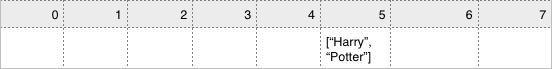
Since I’m writing this with the assumption you know how to implement a hash table, I’ll abstract away all the actual hashing for now. So we start with an empty hash table (aka array).

We hash a key and put the key/value pair in the resulting index. For the purposes of this example, the key “Harry” has hashed to index 5 and we have put the tuple [“Harry”, “Potter”] in index 5 of the hash table.

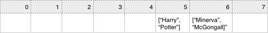
Now, to get to the interesting part, we put another key/value pair into our hash table, and it causes a collision. Key: “Minerva” (with a value of “McGonagall”) happened to hash to index 5 has well.

Instead of using a linked list here, we are going to try to put Minerva McGonagall at another index in the hash table. The change in index needs to be consistent and predictable, so when we go to look up McGonagall, we won’t just stop at the index to which it originally hashed.

For the purposes of simple implementation, we’re going to add 1 to the index and put McGonagall at index 6. This is called linear probing. To fully support this implementation, we’ll also implement contingency plans so that insertion after the end of the hash table simply wraps around to the beginning.

To recap: [“Harry”, “Potter”] has been inserted at index 5. [“Minerva”, “McGonagall”] was going to be inserted at index 5, but that index is already occupied, so [“Minerva”, “McGonagall”] will be inserted at index (5 + 1), or 6.

Retrieving Information

When we go to retrieve [“Harry”, “Potter”], we re-hash “Harry” and find the index of 5 again. [“Harry”, “Potter”] is actually in index 5, so that is fine.

There are two things that could happen when we go to retrieve [“Minerva”, “McGonagall”].

• [“Harry”, “Potter”] exists in the index that “Minerva” hashes to, and we have to walk along the hash table to find [“Minerva”, “McGonagall”].

• we have removed [“Harry”, “Potter”] from the hash table and we have to walk along the hash table to find [“Minerva”, “McGonagall”].

In the case of the first option, the answer is relatively simple. If index 5 is occupied and the first value in the tuple is not the same as the key that we’re passing in (ie, tuple[0] !== “Minerva”), we walk along the hash table. When we get to the end of the table, we start over at the beginning.

The second case is slightly more challenging. To clarify: let’s say that, when we remove an item from the hash table, we reset the value of the hash table at that index to undefined. Since there is no way to distinguish an undefined that represents nothing was ever in that index to begin with (and the function won’t need to walk along the hash table to look for the key) and an undefined that represents something was there, but has been removed (and we should walk along the hash table to look for the key), we encounter a problem.

Luckily, there’s a simple solution to the problem. When we remove an item from the hash table, instead of letting the hash table at that index become undefined we simply set it to null or -1. That way, if we remove [“Harry”, “Potter”]…

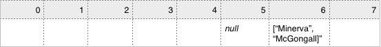
…when we try to retrieve “McGonagall”, the retrieve method will look into index 5 (as originally hashed to), see that something had once been there, and continue looking along the hash table to find “McGonagall”.

So, in essense:

• You insert a value at the index of the hash table that its key, or label, hashed to.

• If another key hashed to that same value, you place it in a different index. You also make sure that the change of index is predictable and consistent, so you can follow the same path to look up the value later.

• If you remove a value, you set that index of the hash table to null or -1, or some other value that the retrieval method will recognize as indicating that a value had once been there.

• When you retrieve a value, if it’s not in its original hashed location, you check other indexes in the hash table (following that predictable and consistent pattern you set earlier) to see if the value you’re looking for is there, if another value is there, if a value had been there but has been removed, or whether no value has been there ever.

Advantages and Disadvantages of Linear Probing

Of course, changing the index by simply adding 1 is a pretty naive way to solve conflict resolution. The lack of randomness creates problems with clustering, or when the indexes are filled for long spans of the hash table and you have to walk through each of those indexes to find a free one.

A better way to implement the same basic idea (that is, to try to insert your value at a different, but predictable index when a conflict occurs) is to have a second hash function that will give us a second number. We add these two indexes together (the one from the first hash function and the one from the second) and, similar to linear probing, if they are greater than the highest index in the hash table, we wrap around to the beginning of the hash table. Then we continue as outlined above.

The sole difference between the in-depth explanation of linear probing above and the second hash function I just mentioned is the number we add to the original index given by the original hash function. If we implement a second hash function, the number it returns will be consistent (every time you hash a key, it will return the same index), but random between different keys. As long as the number of values in the hash table remains less than 75% of the number of indexes available (which is the threshold for all hash tables), this implementation remains effective and efficient, with a time complexity of O(1), just like any other hash table.

Conclusion

That’s it for this blog post! If you would like to read further, Wikipedia has excellent resources for further study. Perhaps check out the article on quadratic probing, or universal hashing, or K-independent hashing. Enjoy!